R for Global Climate forecasting
Joe has a great post on using R for exploiting existing climate datasets to create some really nice weather maps. Using the free information from the U.S. National Centers for Environmental Prediction (NCEP) Global Forecast System (GFS), he shows how R can be used to interpret GRIB2 files after they are pre-processed using wgrib2 (available on MacPorts) to the netcdf format.
I've slightly modified the code from Joe but its pretty much as he wrote it.
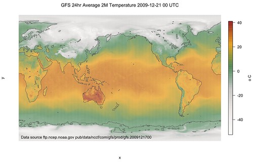
The image continues to show cold conditions in Europe, and the continuing heatwave in Australia.
I've slightly modified the code from Joe but its pretty much as he wrote it.
# ftp.ncep.noaa.gov pub/data/nccf/com/gfs/prod/gfs.2009121700
# See http://www.nco.ncep.noaa.gov/pmb/products/gfs/gfs.t00z.sfluxgrbf00.grib2.shtml
# eoin-brazils-macbook-pro:~ eoinbrazil$ cp gfs.t00z.sfluxgrbf03.grib2 temp2.grb
# wgrib2 was installed using macports
# /opt/local/bin/wgrib2 -s temp2.grb | grep ":LAND:" | /opt/local/bin/wgrib2 -i temp2.grb -netcdf LAND2.nc
# /opt/local/bin/wgrib2 -s temp2.grb | grep ":TMP:2" | /opt/local/bin/wgrib2 -i temp2.grb -netcdf TEMP2.nc
library(ncdf)
landFrac2 <- open.ncdf("LAND2.nc")
land2 <- get.var.ncdf(landFrac2, "LAND_surface")
x <- get.var.ncdf(landFrac2, "longitude")
y <- get.var.ncdf(landFrac2, "latitude")
library(fields)
rgb.palette <- colorRampPalette(c("snow1","snow2","snow3","seagreen","orange","firebrick"), space = "rgb")
tempFrac2 <- open.ncdf("TEMP2.nc")
temp2 <- get.var.ncdf(tempFrac2, "TMP_2maboveground")
newtemp2 <- temp2-273.15 # Convert the kelvin records to celsius
image.plot(x,y,newtemp2,col=rgb.palette(200),axes=F,main=as.expression(paste("GFS 24hr Average 2M Temperature 2009-12-21 00 UTC",sep="")),legend.lab="o C")
contour(x,y,land2,add=TRUE,lwd=1,levels=0.99,drawlabels=FALSE,col="grey30") #add land outline
text(120,-85,"Data source ftp.ncep.noaa.gov pub/data/nccf/com/gfs/prod/gfs.2009121700")
The image continues to show cold conditions in Europe, and the continuing heatwave in Australia.
Labels: GFS, netcdf, R, weathermaps
posted by Eoin Brazil at
1:19 am
![]()


0 Comments:
Post a Comment
<< Home